Lab 3: Closed Loop Control

Overview

In this lab, we are going to apply closed-loop control to trajectory tracking. A ROS Subscriber is included in the script to receive real-time odometry feedback from Gazebo simulator. With the odom/pose updates, the robot can adjust its moving direction accordingly and check if the desired waypoint has been reached.

Specifically, the task is to implement a PD controller (a variant/subset of PID controller) to track the square shape trajectory. Same as in Lab 2, the waypoints are [4, 0], [4, 4], [0, 4], [0, 0], and the sequence does matter. After task completion, the robot should stop at the origin and the Python script should exit gracefully. Please plot the trajectory (using another provided Python script) and discuss your results in the lab report.

To help you complete the lab, please take a look at the Classes section in Python Docs.

Preview

We will play with manipulators in the simulation next time. (Specifically, to solve a Forward Kinematics and an Inverse Kinematics problem.) Note that we will start to team up in Lab 4, so please try to form your team ASAP.

Submission

Submission: individual submission via Gradescope
Demo: required during the lab session (will use autograder; see below)
Due time: 23:59pm, Nov 3, Friday
Files to submit: (please use exactly the same filename; case sensitive)
- lab3_report.pdf
- closed_loop.py
Grading rubric:
- + 30% Clearly describe your approach and explain your code in the lab report.
- + 20% Plot the trajectory and discuss the results of different values of Kp and Kd.
- + 40% Implement PD controller; visit four vertices of the square trajectory with error < 0.1m. Partial credits will be given according to the number of vertices visited.
- + 10% The script can complete the task on time and exit gracefully.
- - 15% Penalty applies for each late day.

Autograder

All code submissions will be graded automatically by an autograder uploaded to Gradescope. Your scripts will be tested on a Ubuntu cloud server using a similar ROS + Gazebo environment. The grading results will be available in a couple of minutes after submission. For the M1/M2 architecture computers, please provide your final code and video of the robot behavior, as I will be tested offline.

Testing parameters are as follows.

The tolerance for distance error is set to 0.1m (considering that this is closed-loop control).
- For example, passing point [3.96, 3.94] is approximately equivalent to passing point [4, 4].
The required waypoints for square trajectory are [4, 0], [4, 4], [0, 4] and [0, 0]; sequence matters.
The time limit for the submitted script is set to 5 mins.
- If running properly, the task in this lab can be done in about 2 mins, based on testing.
- If running timeout, the script will be terminated and a 10% penalty will apply.

Note

It is required to use closed-loop control (i.e. PD controller) to track the trajectory. Finely tuned open-loop control script may also pass the autograder tests (by adding angular velocity as in Lab 2) but is not allowed. All scripts will be double checked when grading manually. Penalty will apply if such script is found.

PID Control

Consider the following feedback control diagram.

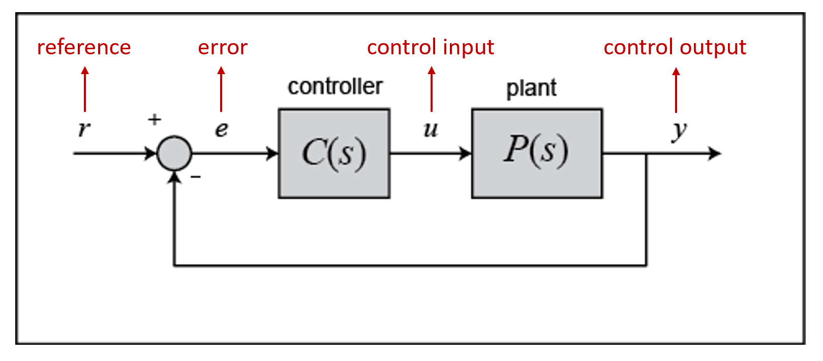
The plant is the system we would like to control. In our case, the control input u is the velocity command we send to the robot, the control output y is the current state (2D pose: x, y, theta) of the robot, and the reference r is the desired state we would like the robot to reach.
The controller is what we need to design. It takes in the tracking error e, which is the difference between the desired reference r and the actual output y, and computes the control input u according to the following equation. (The control input to the plant is the output of the controller.)

\[\begin{equation*} u(t) = k_p e(t) + k_i \int e(t)dt + k_d \frac{de(t)}{dt} \end{equation*}\]

This equation reveals the name of the controller: Proportional–Integral–Derivative (PID) controller, because it has three terms: proportional term, integral term and derivative term. In each term, we have a coefficient k multiplies the (integral/derivative of the) error. The Kp, Ki, and Kd are the coefficients/parameters we need to tune.
In math, it has rigorous analysis to show the stability and convergence of the system, which can be used to calculate the optimal parameters Kp, Ki and Kd. (This should be covered in EE132 Automatic Control course. See this PID Controller Design tutorial for more information.) However, in this lab manually tuned non-optimal parameters are sufficient to complete the task. You may start with some value close to 1 for Kp and a smaller value for Kd.
As for the integral and the derivative of the error, in discrete systems, we can replace integral with summation and replace derivative with subtraction.

\[\begin{equation*} u(t) = k_p e(t) + k_i \sum e(t) + k_d \frac{e(t) - e(t-\Delta t)}{\Delta t} \end{equation*}\]

Due to the negative effect from integral component, we will drop this term and only focus on PD controller. Also, the time inverval \(\Delta t\) can be merged into parameter Kd. (If we run at 10Hz, the time inverval will be 0.1 second.) Therefore, we have the following equation ready, which is what you need to implement in this lab.

\[\begin{equation*} u(t) = k_p e(t) + k_d (e(t) - e(t-\Delta t)) \end{equation*}\]

A discrete PD controller implementation in Python is provided for your information. (You may or may not use it in your own implementation.) To make it work, you need to understand the PD control algorithm and complete the three lines of code under the update function.

class Controller:
    def __init__(self, P=0.0, D=0.0, set_point=0):
        self.Kp = P
        self.Kd = D
        self.set_point = set_point # reference (desired value)
        self.previous_error = 0

    def update(self, current_value):
        # calculate P_term and D_term
        error = 
        P_term = 
        D_term = 
        self.previous_error = error
        return P_term + D_term

    def setPoint(self, set_point):
        self.set_point = set_point
        self.previous_error = 0
    
    def setPD(self, P=0.0, D=0.0):
        self.Kp = P
        self.Kd = D

Programming Tips

Note that the orientation of the robot (theta) ranges from -pi to pi on 2D plane. When the robot turns in CCW direction and passes the direction of negative x axis, the value of theta will jump from pi to -pi. This needs to be handled properly, otherwise the robot will keep turning in place and cannot move forward. It is recommended that you bring up a robot, turn in place using keyboard teleoperation, and see how the value changes for theta. (You can see it from ROS logging messages if using the provided closed_loop.py file).
In general, PID controller is used to track a certain target value (called setpoint), and make sure the system can converge to this target value. For example, to control the temperature in a boiler system. (Note that the setpoint is a scalar, set to a certain target value.)
In our case, we have three variables (x, y, theta) to describe the 2D pose of the robot. At one time only one of them can be set as the desired value to track in a PID controller. If you are willing to track x, y, and theta at the same time, you will need three PID controllers. (To comlpete the task in this lab, out of three controllers, the one to track theta is required, and the other two for x and y are optional. See below an example algorithm.)
The following is an example of how to apply feedback control algorithm to waypoint navigation problem. You may follow this algorithm to start your implementation.

Suppose the robot’s current orientation is \(\theta\), the desired orientation is \(\theta^*\), the current position on X-Y plane is \((x, y)\), and the desired position on X-Y plane is \((x^*, y^*)\).
Calculate the moving direction from the difference between \((x, y)\) and \((x^*, y^*)\); set it as the desired orientation \(\theta^*\).
Initialize a PID controller with the setpoint \(\theta^*\) and a set of parameters (Kp, Ki and Kd). Adjust the angle according to the angular velocity computed by the PID controller.
Once \(\theta \rightarrow \theta^*\), start moving forward at a constant speed (or using a linear velocity generated by another PID controller), and keep adjusting the angle and checking the remaining distance toward desired position \((x^*, y^*)\).
Once \((x, y) \rightarrow (x^*, y^*)\), stop and repeat the process for the next waypoint.

Sample Code

A sample code is provided as the starting point for your implementation. Please read carefully the provided code, and understand its functionality.

Open a new terminal and go to the ee144f23 package. We will start from a new python script.
```
roscd ee144f23/scripts
touch closed_loop.py
gedit closed_loop.py
```

Please copy and paste the following code, then save and close it. If you are using M1/M2, please replace the ROS Topic with “cmd_vel”.

#!/usr/bin/env python

from math import pi, sqrt, atan2, cos, sin
import numpy as np

import rospy
import tf
from std_msgs.msg import Empty
from nav_msgs.msg import Odometry
from geometry_msgs.msg import Twist, Pose2D

class Turtlebot():
    def __init__(self):
        rospy.init_node("turtlebot_move")
        rospy.loginfo("Press Ctrl + C to terminate")
        self.vel_pub = rospy.Publisher("cmd_vel_mux/input/navi", Twist, queue_size=10)
        self.rate = rospy.Rate(10)

        # reset odometry to zero
        self.reset_pub = rospy.Publisher("mobile_base/commands/reset_odometry", Empty, queue_size=10)
        for i in range(10):
            self.reset_pub.publish(Empty())
            self.rate.sleep()
        
        # subscribe to odometry
        self.pose = Pose2D()
        self.logging_counter = 0
        self.trajectory = list()
        self.odom_sub = rospy.Subscriber("odom", Odometry, self.odom_callback)

        try:
            self.run()
        except rospy.ROSInterruptException:
            rospy.loginfo("Action terminated.")
        finally:
            # save trajectory into csv file
            np.savetxt('trajectory.csv', np.array(self.trajectory), fmt='%f', delimiter=',')


    def run(self):
        # add your code here to adjust your movement based on 2D pose feedback
        # Use the Controller
        pass


    def odom_callback(self, msg):
        # get pose = (x, y, theta) from odometry topic
        quarternion = [msg.pose.pose.orientation.x,msg.pose.pose.orientation.y,\
                    msg.pose.pose.orientation.z, msg.pose.pose.orientation.w]
        (roll, pitch, yaw) = tf.transformations.euler_from_quaternion(quarternion)
        self.pose.theta = yaw
        self.pose.x = msg.pose.pose.position.x
        self.pose.y = msg.pose.pose.position.y

        # logging once every 100 times (Gazebo runs at 1000Hz; we save it at 10Hz)
        self.logging_counter += 1
        if self.logging_counter == 100:
            self.logging_counter = 0
            self.trajectory.append([self.pose.x, self.pose.y])  # save trajectory
            # display (x, y, theta) on the terminal
            rospy.loginfo("odom: x=" + str(self.pose.x) +\
                ";  y=" + str(self.pose.y) + ";  theta=" + str(yaw))


if __name__ == '__main__':
    whatever = Turtlebot()

Please make changes to the run function to complete the task in this lab. Once finished, you can run it two ways as introduced in Lab 2. (Remember to bring up the robot before running the script.)
```
python closed_loop.py
```
```
chmod +x closed_loop.py
./closed_loop.py
```

Sample Code Explained

Odometry works in the way that it counts how many rounds the wheel rotates. Therefore, if you lift and place a robot from one place to another, it will still “think” that it is at the original place.
In Gazebo simulator, using command Ctrl + R to reset the robot is similar to lifting the robot and placing it to the origin, where the odometry will still report the previous history record. Therefore, to obtain a correct odometry feedback for the new run, we need to reset the odometry to zero.
```
self.reset_pub = rospy.Publisher("mobile_base/commands/reset_odometry", Empty, queue_size=10)
for i in range(10):
    self.reset_pub.publish(Empty())
    self.rate.sleep()
```
In Lab 2, we have learned how to use ROS Publisher to send a message out. ROS Subscriber is the one on the other side to receive and process the messages. The required arguments are the topic name odom, the message type Odometry, and a pointer to the callback function. The callback function will be executed whenever a new message is received (asynchronously; in another thread). We leverage the shared variables in Turtlebot class to store the latest pose of the robot. Note that the msg argument in the callback function is of the type Odometry. The definition is specified in the ROS Wiki documentation.
```
self.odom_sub = rospy.Subscriber("odom", Odometry, self.odom_callback)

def odom_callback(self, msg):
    pass
```
In the try-except structure, finally is the keyword to indicate that the following code block will be executed regardless if the try block raises an error or not. In this case, we want to save the trajectory even when the robot stops halfway.
```
finally:
    # save trajectory into csv file
    np.savetxt('trajectory.csv', np.array(self.trajectory), fmt='%f', delimiter=',')
```

Visualization

We provide a separate Python script to help visualize the trajectory from the saved csv file. Please do not submit this file and do not include it in the script you plan to submit, as it will block the autograder until running timeout.

#!/usr/bin/env python

import numpy as np
import matplotlib.pyplot as plt

def visualization():
    # load csv file and plot trajectory 
    _, ax = plt.subplots(1)
    ax.set_aspect('equal')

    trajectory = np.loadtxt("trajectory.csv", delimiter=',')
    plt.plot(trajectory[:, 0], trajectory[:, 1], linewidth=2)

    plt.xlim(-1, 5)
    plt.ylim(-1, 5)
    plt.show()

if __name__ == '__main__':
    visualization()