Lab 6: Trajectory Generation

Overview

In this lab, we will focus on how to generate smooth trajectories using polynomial time scaling.

Specifically, the task is to implement the 3rd order polynomial time scaling and apply it for each segment of the trajectory and for both x and y coordinates. Waypoints will be provided in the sample script, and should be included in the boundary/continuity constraints when generating trajectories.

Preview: Next time we will learn how to use A* algorithm to search for the waypoints, when a map is given.

Submission

Submission: group submission via Gradescope. Important: If any of the two team members have ROS Kinetic installed, it is highly recommended to setup the code on this computer and not on the M1/M2 computer. The main reason for this is that during the final Lab 8, the real turtlebots have ROS Kinetic installed so there will be fewer code modifications if you develop your ROS nodes for ROS Kinetic.
Demo: not required
Due time: 11:59pm, Nov 27, Monday
Files to submit:
- lab6_report.pdf (please include the plot of trajectory)
- trajectory_generation.py
Grading rubric:
- + 30% Clearly describe your approach and explain your code in the lab report.
- + 20% Plot the trajectory and discuss the results under different parameters.
- + 50% Pass all waypoints using 3rd order polynomial trajectories.
- - 15% Penalty applies for each late day.

Autograder

All code submissions will be graded automatically by an autograder uploaded to Gradescope. The scripts will be tested on a Ubuntu cloud server using a similar ROS + Gazebo environment. The grading results will be available in a couple of minutes after submission.

Testing parameters are as follows.

The tolerance for distance error is set to 0.1m.
- For example, passing point [3.96, 3.94] is approximately equivalent to passing point [4, 4].
The autograder will check 8 out of 14 waypoints and the last stopping point [0, 0].
- They are [0.5, 0], [0.5, -0.5], [0.5, 0.5], [1, 0], [1, -0.5], [1, 0.5], [1.5, -0.5], [1.5, 0.5].
The time limit is set to 5 mins.

Sample Code

Open a new terminal and go to your ee144f23 package. We will start from a new python script.
```
roscd ee144f23/scripts
touch trajectory_generation.py
gedit trajectory_generation.py
```

Please copy and paste the following code. If both of the team members have an M1/M2 computer, please follow the corresponding approach by replacing the Python version with ‘’python3’’ and the ROS Topic with “cmd_vel”.

#!/usr/bin/env python

from math import pi, sqrt, atan2, cos, sin
import numpy as np

import rospy
import tf
from std_msgs.msg import Empty
from nav_msgs.msg import Odometry
from geometry_msgs.msg import Twist, Pose2D


class Turtlebot():
    def __init__(self):
        rospy.init_node("turtlebot_move")
        rospy.loginfo("Press Ctrl + C to terminate")
        self.vel_pub = rospy.Publisher("cmd_vel_mux/input/navi", Twist, queue_size=10)
        self.rate = rospy.Rate(10)

        # reset odometry to zero
        self.reset_pub = rospy.Publisher("mobile_base/commands/reset_odometry", Empty, queue_size=10)
        for i in range(10):
            self.reset_pub.publish(Empty())
            self.rate.sleep()
        
        # subscribe to odometry
        self.pose = Pose2D()
        self.logging_counter = 0
        self.trajectory = list()
        self.odom_sub = rospy.Subscriber("odom", Odometry, self.odom_callback)

        try:
            self.run()
        except rospy.ROSInterruptException:
            rospy.loginfo("Action terminated.")
        finally:
            # save trajectory into csv file
            np.savetxt('trajectory.csv', np.array(self.trajectory), fmt='%f', delimiter=',')


    def run(self):
        waypoints = [[0.5, 0], [0.5, -0.5], [1, -0.5], [1, 0], [1, 0.5],\
                      [1.5, 0.5], [1.5, 0], [1.5, -0.5], [1, -0.5], [1, 0],\
                      [1, 0.5], [0.5, 0.5], [0.5, 0], [0, 0], [0, 0]]
        for i in range(len(waypoints)-1):
            self.move_to_point(waypoints[i], waypoints[i+1])


    def move_to_point(self, current_waypoint, next_waypoint):
        # generate polynomial trajectory and move to current_waypoint
        # next_waypoint is to help determine the velocity to pass current_waypoint
        pass


    def polynomial_time_scaling_3rd_order(self, p_start, v_start, p_end, v_end, T):
        # input: p,v: position and velocity of start/end point
        #        T: the desired time to complete this segment of trajectory (in second)
        # output: the coefficients of this polynomial
        pass


    def odom_callback(self, msg):
        # get pose = (x, y, theta) from odometry topic
        quarternion = [msg.pose.pose.orientation.x, msg.pose.pose.orientation.y,\
                    msg.pose.pose.orientation.z, msg.pose.pose.orientation.w]
        (roll, pitch, yaw) = tf.transformations.euler_from_quaternion(quarternion)
        self.pose.theta = yaw
        self.pose.x = msg.pose.pose.position.x
        self.pose.y = msg.pose.pose.position.y

        # logging once every 100 times (Gazebo runs at 1000Hz; we save it at 10Hz)
        self.logging_counter += 1
        if self.logging_counter == 100:
            self.logging_counter = 0
            self.trajectory.append([self.pose.x, self.pose.y])  # save trajectory
            rospy.loginfo("odom: x=" + str(self.pose.x) +\
                ";  y=" + str(self.pose.y) + ";  theta=" + str(yaw))


if __name__ == '__main__':
    whatever = Turtlebot()

This script is following the same structure as the one used in Lab 3, except for the changes under run function.
You need to complete the move_to_point function in this code, and make sure the robot can pass all the waypoints. The polynomial_time_scaling_3rd_order function is provided for your information only. You may or may not use it.

Polynomial Time Scaling

Suppose that we have figured out a path from point A to point B. The question is how fast the robot should follow the path (i.e. where it should be at each moment). This process of generating intermediate points (each associated with a time stamp) is called time scaling, or trajectory generation at large.

Recall that sending constant velocity commands from the very beginning would assume the robot can have infinite large acceleration at the first moment, which is impractical. Therefore, we would like to have a smooth trajectory that can best fit robot kinematics.

On the other hand, polynomial functions are smooth (infinitely differentiable) functions that can provide us smooth trajectories at all orders (position, velocity, acceleration, the derivative of acceleration, and so on). To this end, polynomial time scaling becomes a good choice to generate trajectories.

Suppose that we plan to move from point A to point B in T seconds by following a straight line. Then where the robot should be at each moment can be described by the following function. It provides the position of the robot x(t) at any given time t.

\[\begin{equation} x(t) = a_{0} + a_{1} t + a_{2} t^{2} + a_{3} t^{3}, t \in [0, T] \end{equation}\]

Accordingly, the expected velocity at any time t can be described by the derivative of this polynomial function.

\[\begin{equation} \dot{x}(t) = a_{1} + 2 a_{2} t + 3 a_{3} t^{2}, t \in [0, T] \end{equation}\]

The key is to figure out the coefficients of this function for each and every trajectory segment and for both x and y coordinates. In other words, coefficients can vary from segment to segment, as each segment should adopt different initial and terminal conditions to best fit its needs.

Fortunately, we can formulate this problem into a linear system of equation as follows, where \(x_0, x_T, \dot{x}_0, \dot{x}_T\) are initial/terminal position/velocity respectively.

\[\begin{split}\begin{equation} \left[\begin{array}{c} x_{0} \\ x_{T} \\ \dot{x}_{0} \\ \dot{x}_{T} \end{array}\right]=\left[\begin{array}{cccc} 0 & 0 & 0 & 1 \\ T^{3} & T^{2} & T & 1 \\ 0 & 0 & 1 & 0 \\ 3 T^{2} & 2 T & 1 & 0 \end{array}\right]\left[\begin{array}{l} a_{3} \\ a_{2} \\ a_{1} \\ a_{0} \end{array}\right] \end{equation}\end{split}\]

To solve this equation of the form \(x = Ta\), we can simply take the advantage of the inverse matrix and have the solution \(a = T^{-1}x\). Once the coefficients are known, the position and the velocity at each moment can be obtained by evaluating the function \(x(t)\) and \(\dot{x}(t)\) at \(t = 0, 0.1, 0.2, ..., T\). (This is an example of running at 10Hz where the time interval is 0.1s.)

Finally, a PID controller (introduced in Lab 3) can be applied to track the desired position and velocity at each moment. To closely track the trajectory, the parameter Kp can take a larger value. As before, it is possible to only track the orientation by the PID controller and simply set the linear velocity to be the magnitude (i.e. \(v = \sqrt{v_x^2 + v_y^2}\) ). Note that the orientation setpoint in this lab is changing all the time as the robot follows the trajectory (as opposed to a fixed setpoint in Lab 3).

So far we have introduced the basic steps to solve for a polynomial time scaling problem. The following are three final remarks regarding the selection of parameters.

Two ways to pick the time interval T (this is one of the drawbacks of this approach; you have to specify T ahead of time)
- Fixed time interval for all segments.
- Pick a preferred average speed, then determine T based on the distance to travel.
Notes on boundary conditions and continuity constraints
- It is better to look at not only the current waypoint, but also the next one. Because normally the next waypoint can provide useful information to help determine how to pass the current waypoint.
- For example, when moving from point A to point B by following a straight line, knowing that point C is to the right of point B is a good indicator to curve the current trajectory a bit more, such that this turning behavior can be evenly distributed in the trajectory and avoid a sharp turn at point B.
- In practice, the magnitude of the velocity can be set to a preferred speed, and the direction of the velocity of passing point B can be set to the direction from point A to point C.
Discussion on the numerical stability of polynomial functions
- It is possible to use a continuous timeline for all trajectories (i.e. \([0, T_1]\) for the first segment, \([T_1, T_2]\) for the second, and so on). However, this approach is not numerically stable, especially when the order of the polynomial is higher.
- For example, in a 7th order polynomial function, as \(T\) grows larger, to make the term \(a_7 t^7\) reasonably small, the parameter \(a_7\) will have to be at the level of \(10^{-10}\) or even smaller.
- Conclusion: we recommend using relative time scale \([0, T]\) for all segments (i.e. reset timing every time).

Visualization

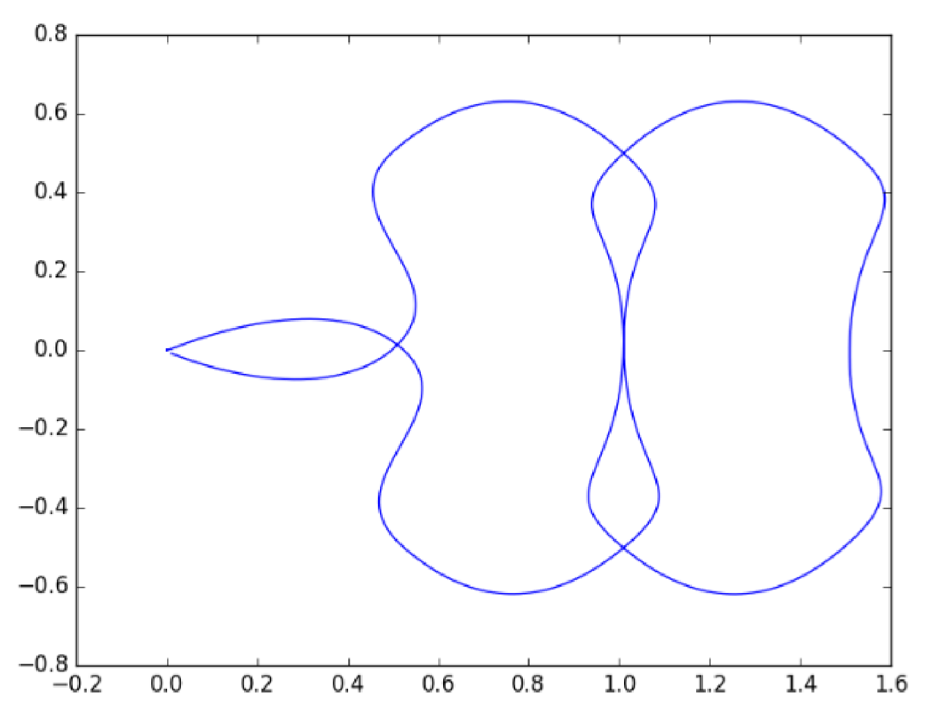
You can reuse the visualization python script provided in Lab 3 to plot the trajectory. Remember to adjust the limit on x and y axes and include the plot in the lab report.
An example of the trajectory is provided as follows. It is a bit overshooting. You can do better :)